How we built high speed threat hunting for email security

The need for quickly analyzing historical data spans security teams. SOC, incident response, and intelligence teams perform threat hunts to investigate attacks and compromises. Detection engineers perform backtesting to test the performance and efficacy of detection rules. In these cases, every second spent waiting for a query response is a second that an attack could be landing and expanding.

Sublime is one of the few email security platforms to offer both historical threat hunting and detection backtesting. We can do this because Sublime is built on Message Query Language (MQL), a domain-specific language purpose-built for querying email data. And as an email security solution for some very large enterprises, we need to be able to do both at speed and scale.

In this post, we’ll take a look at how Sublime is able to process millions of messages in a timely fashion without degrading the product experience.

Things to know before we start

The first thing to know is that, on the backend, both hunts and backtests are the same thing to Sublime. They just get different presentation layers. So for the rest of this post, we’ll just use the word “hunt” to mean both.

The next thing to know is that Sublime splits email data out across warm and cold storage. Lightweight metadata is stored in warm storage and bulkier data (blobs, attachments, raw HTML, etc.) is stored in cold storage. To keep things fast, we query in warm storage first to reduce the amount of requests that will eventually be sent to cold storage. Then to make cold storage operations faster, we parallelize as much as possible.

Now that you have the TL;DR, let’s get into how we do it.

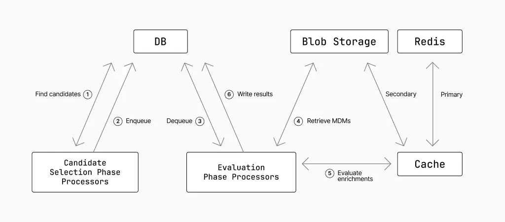
Hunt operationalization: candidates and evaluations

Not all MQL is created equal. Some of its operations are relatively cheap (simple queries), and some are relatively expensive (enrichments). For efficiency’s sake, we run cheap operations first and then only run expensive operations on the subset of messages returned by the cheap operations. We do this by splitting hunts into two phases: the candidate selection phase and the evaluation phase.

In the candidate selection phase, we find relevant messages by querying a database that stores a partial set of the data from each email (more on that in a bit). These candidates are then passed to the evaluation phase to be retrieved and processed. In practice, this happens concurrently and across many workers/processors.

Email ingestion: rows and blobs

As we process emails, a message is saved in the Sublime platform for up to 30 days so it can be hunted over later. This means we not only need to securely save the entire email for arbitrary analysis later, but we also need a way to find relevant messages quickly.

We do this by storing the partial MDM in a database (fast) and the corresponding email in blob storage (complete). In the case of the blob storage, we first parse the raw EML into an easily queryable format called an MDM (Message Data Model) file.

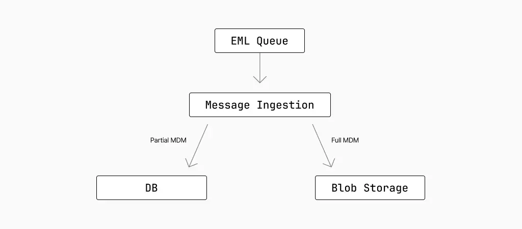
Partial MDM

Here is a simplified version of the kind of common MDM fields we write to the database:

Blobs

MDMs are saved to blob storage with the path format of:

/YYYY/MM/DD/mdms//...//

The date portion of the path refers to the received_at time which makes it easier to prune in the future. The <hash_char_*> portion of the path acts like a trie for the hash of the id to prevent throttling of the path prefix. The trie also helps with navigation to prevent having millions of entries at the /YYYY/MM/DD/mdms path. This means we can derive the blob storage path from just received_at and id.

We store the MDMs as flatbuffers to allow for partial deserialization in the evaluation phase, but we’ll get into that later.

Candidate selection

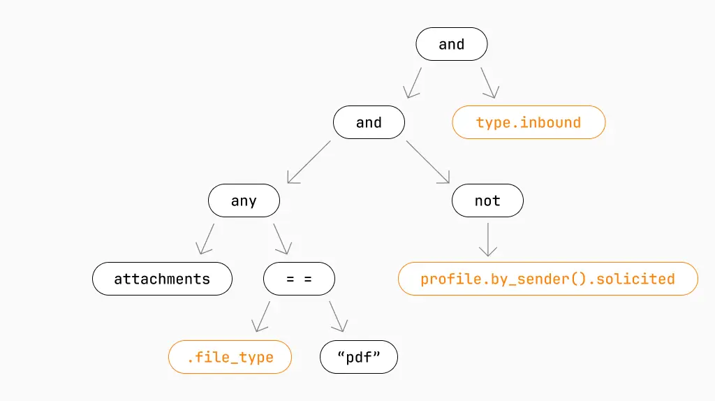
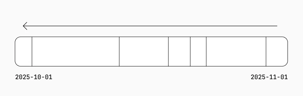
To explain how hunts work, let’s look at an example. Imagine you want to investigate all messages with PayPal invoices coming from unsolicited senders in October 2025.

You could write a hunt like this:

type.inbound
and not profile.by_sender().solicited
and any(attachments,
        .file_type == "pdf"
        and any(ml.logo_detect(.).brands,
                .name == "PayPal" and .confidence == "high"
        )
)

When you click Hunt, Sublime takes that MQL query and does a few things in the background before it returns your results.

SQL generation

After the MQL is parsed and validated, it's turned it into this intermediate representation (IR). This is the simplified version:

MQL knows that the nodes highlighted in orange can be found in the database. This means we can compile a portion of the IR to SQL to find eligible messages, instead of having to process every single message in the hunt timeframe. This is done using predicate pushdown, the core technique that powers index scans for most databases.

It’s important to remember that this is just the candidate selection IR, so it only needs to return a candidate set that’s free of false negatives. False positives are fine in this phase, as the evaluation phase will filter them out later.

Here is the IR that can be compiled to SQL:

This roughly compiles to:

SELECT id, received_at
FROM mdms
WHERE received_at >= '2025-10-31'
	AND received_at < '2025-11-01'
	AND "type.inbound"
	AND 'pdf' = ANY(attachment_file_types)
	AND NOT EXISTS (
		SELECT 1
		FROM sender_history
		WHERE sender_history.email = mdms.sender_email
			-- We only want the history up to when we received the message
			AND sender_history.received_at < mdms.received_at
			AND sender_history.solicited
	)

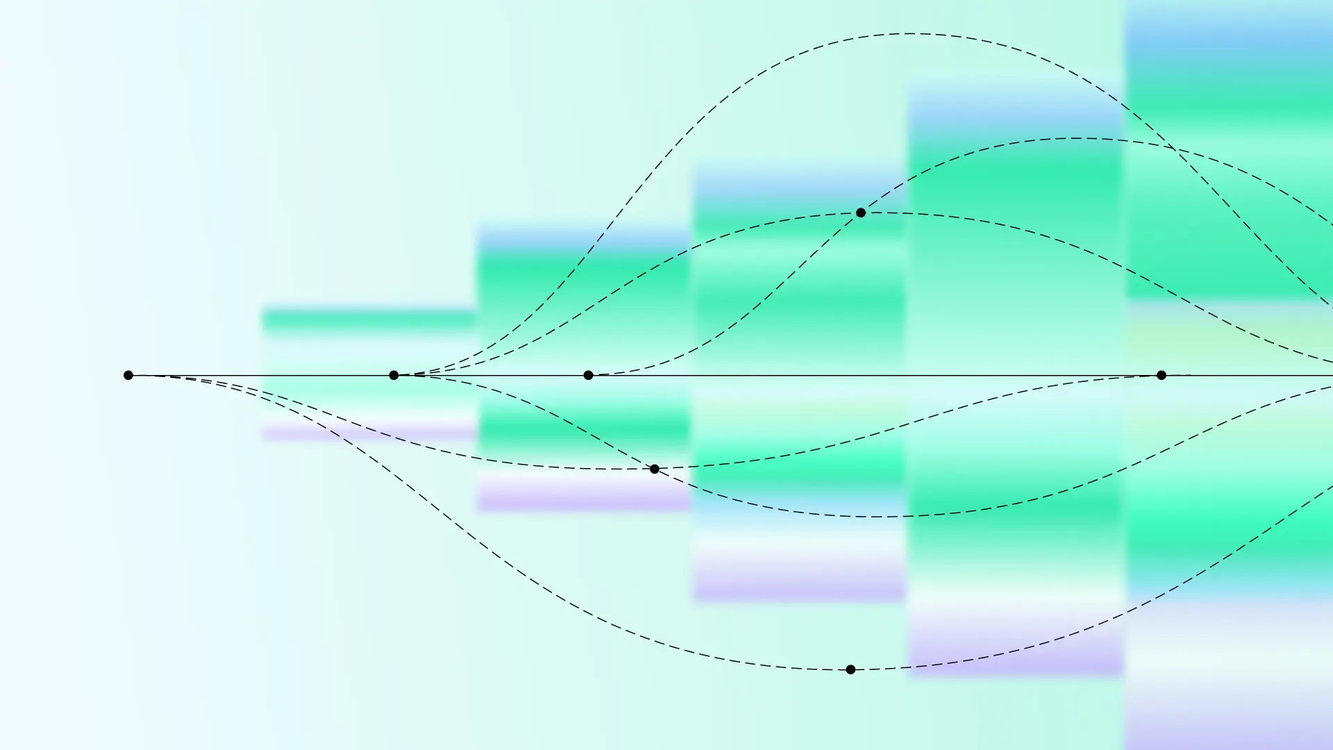
Period chunking

Did you notice that in the query above that we’re only looking at a single day in October instead of the entire month? This is because we split the hunt timeframe up into chunks called periods.

By splitting the hunt into periods, we can process candidate messages sooner and in parallel in order to get results to the user quicker. This means we don’t have to wait for all candidates to be selected before processing can begin.

Chunking goes in reverse chronological order (newest to oldest) because we want to surface recent messages as soon as possible in order to address an immediate incident. The theory is that a problematic email that came in yesterday is much more relevant than one that came in a month ago (e.g. URL payloads are often dead well before 30 days).

In the example, the period is shown as a day. In practice, we dynamically size these periods using an exponentially weighted moving average of the query execution time. The main reasons for this are:

• Email activity is spiky (e.g. Monday morning vs the weekends), so we need to adjust the period size to maintain consistent performance across the entire hunt timeframe.
• Hunts need to self-throttle when the database is under load or go faster when more DB resources are available.
• Hunts need to auto-adjust if the query is easily indexable. Queries that require O(n) behavior can have smaller batches but queries with indexes can efficiently search over much larger periods.

We accomplish this by setting a target query duration range of 5-15 seconds and weighing newer query execution times more in the moving average to react quickly to DB load. We even set the maximum rate of growth to smooth out the resizing of periods

Evaluation phase

As candidate messages are pulled off the queue, we evaluate the remaining MQL against the MDMs in Go, which eliminates any false positive candidates. This ensures that after this final phase, only MDMs that match the hunt exactly are streamed as results to the user.

Here is the remaining portion of the IR:

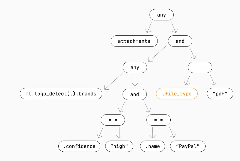
Let’s explore how this evaluation phase IR boosts efficiency and speed. First off, you’ll note that we’re checking .file_type again. This prevents us from running ml.logo_detect on attachments that aren’t PDFs to maintain correctness.

Next, having a reduced IR means that we know exactly which fields we’ll need to deserialize (similar to field masks in protobufs). In our example, we know that we only need .file_type and the raw bytes from attachments in the MDM, so we can ignore everything else. This saves a lot of CPU and memory with each message we process.

Then we fetch our MDMs from blob storage (stored as flatbuffers) and deserialize based on the field mask generated from the evaluation phase IR. All this means we only apply ml.logo_detect to the relevant PDFs and write the results to the database.

On top of that, to evaluate enrichments like ml.logo_detect without causing excessive pressure on downstream services or caching indefinitely, we employ a two tier caching system. Redis acts as a short-lived primary cache for high throughput and blob storage is the long-lived secondary cache to warm up the primary cache again. If a full cache miss does occur, we have concurrency limits in place to prevent a thundering herd of requests.

We’re glossing over many details of our caching strategy (a great topic for a future blog), but all this is to say that a great deal of thought went into maximizing the speed of hunts.

Hurdles along the way

While building the candidate selection phase, we hit a few roadblocks that we needed to resolve to hit our targets for fast hunts. We wanted to share a few here.

Issue #1: Querying around dead tuples

‍The candidate selection phase processor coordinates work with other processors by using a persistent database-backed queue. As a note, we elected to leverage the database to provide strict ordering and durable queues, without major architectural changes – one of the challenges operating as a SaaS and on-prem solution simultaneously.

One major issue the database introduces is that “popping” a pending message off the queue in PostgreSQL will simply mark a tuple as dead, but keep it around until a vacuum can occur. The traffic on this table is so high that the DB never gets the chance to perform a vacuum, so all queries are forced to skip over dead tuples to get to a live one. Ultimately, this turns dequeuing into a table scan even though you would expect to read a single row. We found this by tracking the CPU usage of the query in conjunction with query plans.

Solution: We addressed this issue by saving a cursor of the last known live message ID, which we have indexed, so we can always skip over any prior dead tuples that have yet to be cleaned up. The cursor is cached in-memory for each instance and refreshed periodically from the database in the background. We designate the first processor (based on the assigned ID) to update the cursor in the database to prevent redundant work.

Issue #2: So many stats

‍Another similar issue arose when processors were frequently writing their stats out to the DB. Depending on the hunt, processors could quickly process messages and record the associated stats to the DB in a high volume. Each processor has a single row that it updates for stats but, under the hood, PostgreSQL will treat updates as a deletion and insertion due to multiversion concurrency control (MVCC). This means that a single row could internally be stored as a series of many dead tuples with a single live tuple at the end. The database will spend extra CPU traversing over the dead tuples in search of the live one similar to a sequence scan.

Solution: We addressed this by adding a new updated_at column that we indexed so we could use the most recent updated_at for that row to find a live tuple, which is still useful even though it's only one row. The index allows us to fully skip over old versions of the row that haven’t been vacuumed yet.

Issue #3: Naive processors

‍Initially, every processor would naively query the DB to refresh their state of the hunt in order to determine whether they needed to continue processing. As we scaled up the number of processors per hunt, we encountered excessively high DB load and contention.

Solution: Similar to updating the cursor, we designate the first processor to aggregate stats and make it available to other processors (either through Redis or a pre-aggregated table). Processor IDs are assigned in ascending order of available IDs so we’ll always have a notion of a “first” processor. This allows us to continue to scale up processors without also scaling up status queries.

Future updates

Our hunts are fast, but there’s always room for improvement. For example, putting too much data in warm storage can max out RAM utilization, which in turn creates cache misses and storage cooling via DB thrashing. To prevent this in the candidate selection phase, we’re currently looking into leveraging lossy data structures (such as bloom filters) for efficient checks that don’t compromise too much storage or performance. Since the evaluation phase will ultimately deal with any false positives, we have some room to exchange precision for performance during candidate selection.

Additionally, we have a static number of phase processors dedicated to each hunt – but each hunt has different demands and bottlenecks. In the future, we will make the number of processors dynamic based on the bottlenecks of the hunt, while also minimizing the affect on other concurrent hunts. For example, during lower DB usage times, we could utilize more DB connections to scale up the number of candidate selection phase processors. We would then scale back down during peak load.

Hunt speed matters

At a high level, we’ve been able to maximize hunt and backtest speed by splitting out the candidate selection and evaluation process and processing both in parallel. This architecture allows us to scale compute to meet enterprise-scale needs without degrading the platform. By digging into bottlenecks, we’ve added a lot of optimizations within this architecture – and we’re going to keep adding more. Our goal is to keep making hunts better and faster so security practitioners have the speed at scale that they’ve come to demand.

If you enjoyed this post, send us your questions and comments over social (LinkedIn, X). And if this is the type of challenge you like tackling, get in touch with our Engineering team.