How to build fast similarity search for email from the ground up

In a previous post, we shared how grouping similar email messages is crucial for an effective and productive analyst experience, as well as for bolstering herd immunity. This is why Sublime automatically groups similar messages before rule processing. It lets us operates on messages at the individual or group level and enables cascading remediation, like automatically quarantining a message when it’s part of an already quarantined group.

Since grouping happens early in message processing, we only have milliseconds to efficiently find prior ingested messages to group with. This is an important foundational component of the Sublime platform and we’re proud of our solution, so we want to share the science and engineering that powers efficient search against a corpus of messages for highly similar, but inexact, matches.

In this engineering deep dive, we’ll cover:

• What message similarity means
• Problems with string similarity at scale
• Representing a message as a set to leverage more similarity algorithms
• Incorporating MinHash and the banding technique for efficient lookups

What is message similarity?

Before diving into grouping algorithms, it’s essential to define what “similar” means for messages. In particular, we’re interested in a high degree of matching content in text fields like the body, sender name, subject, attachment names, and even raw attachment content. This metric must be a composite similarity across several distinct fields that represent a message, e.g. “Message 1 and 2 have 95% similar content overall.”

One naive idea is to treat a message as a single large string. Calculating the similarity between two strings with an algorithm like Levenshtein distance is highly accurate but computationally expensive. Specifically, for two strings $s_1$ and $s_2$, the total runtime to evaluate Levenshtein distance is $O(len(s_1) \times len(s_2))$, which scales abysmally for long strings!

Although improvements like Levenshtein automata help, its $O(len(s_1))$ construction and $O(len(s_2))$ runtime per input string still scales with the size of the entire corpus! That only gets worse as the corpus grows, so we need to get more creative.

Sets, not strings

Suppose that instead of strings, a message is interpreted as a set of many fragments. Set similarity is well defined and is typically measured by the Jaccard index, the overlap between two sets. Formally, this is defined by the intersection over the union of two sets, or $J = \frac{|A \cap B|}{|A \cup B|}$ .

For example, with two sets of numbers: $A =\set{1, 2, 3, 5, 7}$ and $B = \set{1, 3, 5, 7, 9}$:

• The union $A \cup B$ is $\set{1,2,3,5,7,9}$
• The intersection  $A \cap B$ is $A \cap B = \set{1,3,5,7}$
• The corresponding Jaccard index is $J = \frac{|A \cap B|}{|A \cup B|} = \frac{4}{6} \approx 0.67$.

For two pre-sorted sets, we calculate Jaccard by iterating each in parallel, resulting in $O(|s_1| + |s_2|)$. This runtime is comparable to leveraging a Levenshtein automata, but also enables more efficient ways to search an entire corpus of sets for matches above a known threshold. Before exploring these techniques, though, we’ll first need to represent a message as a set.

Representing a message as a set

Representing a message as a set requires breaking it into many smaller, representative fragments or substrings. For strings, this involves tokenizing and shingling, and we need isolation to keep fields distinct in the resulting set.

For a single string, such as “The quick brown fox jumps over the lazy dog”, there are several ways to perform tokenization:

• Individual characters: ["T", "h", "e", " ", "q", "u", ...]
• Words: ["The", "quick", "brown", ...] .

This bag of words model has a weakness to rearrangements. For those interpretations, the same words in two different orders are identical sets. To mitigate this, we take a sliding window over these tokens, employing a technique known as shingling, which is sensitive to local rearrangements. For a sliding window of three tokens, we have the shingles:

• Characters:["The", "he ", "e q", " qu", "qui", ...]
• Words: ["The quick brown", "quick brown fox", "brown fox jumps", ...].

Once all tokens and shingles are generated, the composite set is ready to be constructed and individual elements across fields are isolated. This prevents substrings in the email subject from unintentional comparisons to another field like the sender’s display name. Collectively, this whole one-time process takes $O(len(message))$ to build the final set, which looks like:

{
	// (field, shingle)
	("subject", "Your subscription")
	("subject", "subscription is"),
	("subject", "is ready"),
	("subject", "ready for"),
	("subject", "for renewal"),
	
	...
	
	("body", "Dearest customer"),
	("body", "customer we"),
	("body", "we hope"),
	("body", "you're enjoying"),
	("body", "enjoying your"),
	("body", "your subscription")
	...
}

Approximating set similarity with MinHash

With a runtime of $O(|set_1| + |set_2|)$ , calculating the Jaccard index for two sets is bottlenecked by size for large sets. This limitation is circumvented with MinHash, a technique which probabilistically compresses sets to a fixed size data structure. As a probabilistic data structure, MinHash sacrifices a bit of accuracy for performance in its Jaccard calculation. This loss in accuracy is quantifiable and acceptable for our use case, since “similar messages” is an inherently fuzzy concept.

Binary Jaccard estimator from two ordered sets

MinHash is built with the intuition that if we have a random but deterministic ordering across two sets, we can pick a representative element in a consistent way. Suppose we have two sets, $A$ and $B$, which are each sorted consistently to ensure that there is a total ordering over all the elements in both sets. If we retrieve the first element of each set, what’s the probability that these are the same? Formally, we’re asking, what’s $P[min(A) = min(B)]$?

Because the ordering is random, every element in $A \cup B$ has an equal chance to be the minimum. But a match causing $min(A) = min(B)$ can only happen if the element is in both sets, $A \cap B.$ Thus, for any random ordering:

$$P[min(A) = min(B)] = \frac{|A \cap B|}{|A \cup B|} = J(A, B)$$

This gives us a binary estimator: the minimum value for two sets is equal with a probability of $J(A, B)$. On its own this isn’t very useful, and one noisy boolean doesn’t estimate similarity. If two messages are 80% similar, it’s not enough to rely on a true 80% of the time and false 20% of the time.

The key idea here is that once we impose a random, consistent ordering, we’re not picking random values out of two hats. Instead, the shared ordering guarantees a consistent sampling of values from our two sets. This consistent sampling is foundational for us to build a function that can efficiently calculate $J(A, B) \approx 80\%$.

Approximating Jaccard with multiple samples

With more set orderings, we can draw enough random variables to estimate the actual Jaccard index. By ordering these sets $N$ different ways, we compare $N$ minimum values, and thus have $N$ independent random variables. This collection of independent, unbiased variables is just a Bernoulli distribution, which reproduces Jaccard with expected variance and error rates:

• Jaccard: $J = \frac{count(matches)}N$
• Variance: $\sigma^2 = \frac{J(1-J)}N$
• Expected error (standard deviation): $\epsilon = \sigma$

This means that with more orderings, we draw more random variables, increasing the fidelity and reducing the error of our estimate  as $\frac{1}N$ decreases.

Generating a minimum hash fingerprint

With the Min part covered, let’s dive into the Hash part of MinHash. Instead of retaining and ordering the original set, we use different hash functions or seeds to build a collection of minimum hashes. For each of our $N$ hash functions, we collect the lowest hashed value.

min({
	// hash(seed, (field, shingle))
	hash(seed_1, ("subject", "Your subscription")), // 51872
	hash(seed_1, ("subject", "subscription is")),   // 1293
	hash(seed_1, ("subject", "is ready")),          // 30588
	hash(seed_1, ("subject", "ready for")),         // 46114
	hash(seed_1, ("subject", "for renewal")),       // 26931
	
	...
	
	hash(seed_1, ("body", "Dearest customer")),     // 41822
	hash(seed_1, ("body", "customer we")),          // 6021
	hash(seed_1, ("body", "we hope")),              // 49012
	hash(seed_1, ("body", "you're enjoying")),      // 9413
	hash(seed_1, ("body", "enjoying your")),        // 28433
	hash(seed_1, ("body", "your subscription")),    // 44211
	...
}) // 1293

After collecting N minimum hashes, we have a MinHash fingerprint, which is an array corresponding to the minimum hash of all elements in the set. Every message will become a set and go through the same transformation process, with identical hash functions or seeds, resulting in fingerprints that can be compared element to element.

[
	// min(hash(seed_1)
	1293,
	// min(hash(seed_2)
	8294,
	// min(hash(seed_3)
	44210,
	...
	// min(hash(seed_N)
	17290,
]

To estimate Jaccard similarity on two sets, we just need to count the matches and divide it by the length, a trivial computation.

array_size = 10

a = [1293, 8294, 44210, 26138, 30588, 61954, 18220, 9413, 55310, 17290]
b = [1293, 3011, 48293, 26138, 30588, 61954, 17290, 9413, 55310, 17290]

num_matches = 6
jaccard = 6 / 10 = ~67%

At this point, messages are tokenized, shingled, constructed into sets, and processed with MinHash, resulting in a fingerprint that we can use to rapidly check if two messages are equal. The time to generate these fingerprints is still proportional to the size of individual message contents. Once these fingerprints are constructed, comparing two fingerprints is always $O(|fingerprint|)$, but since the fingerprint is a fixed length, this is effectively $O(1)$!

Optimizing for massive datasets with banding

The ability to quickly compare two message fingerprints is a huge unlock, but we still need to search against millions of messages in milliseconds. Brute force comparing signatures will not cut it at that scale, regardless of how quick one comparison is. We need another technique to reduce the search space.

Our end goal is still: “Find me all messages with 90% or higher similarity to X.” Comparing two fingerprints to calculate Jaccard takes us a step closer, but if the threshold is already known, we can actually optimize for that exact threshold!

How banding reduces the search space

One trick to optimize for an exact threshold starts with non-overlapping “bands” of contiguous elements in our arrays, which are hashed again. The array of N could be split into $b$ bands of $r$ rows (hash functions) per band, and we can search for an exact match in at least one band. To match an entire band, all rows within the band must match exactly. Each band provides a different opportunity to match a different fixed set of hash functions. The probability of matching at least one of these bands is:

$P[match] = 1 - (1-J^r)^b$

Depending on the amounts of bands vs rows, we get different recall curves. Below, we’ve graphed different parameters of $b$ and $r$ for $n = b \times r = 120$, which is highly composite and gives many different configurations. On the x-axis is the Jaccard index between two messages and the y-axis is the probability that at least one band is a match.

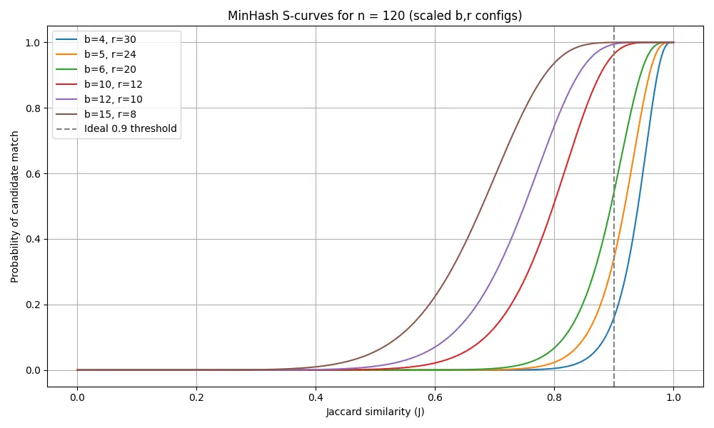
Looking at these results, we see how different values of $b$ and $r$ interact, and how they approximate the ideal step function, where we get only the matches above our threshold of 0.9. Increasing $b$ results in more potentially matched bands (“shifting”  the curve), and increasing $r$ makes it more difficult to match a given band (“steepening” the curve). Together, $b \times r$ equals the total number of hash functions and the size of the fingerprint.

Choosing the fingerprint size $n$, along with the constants $b$ and $r$, is a balance between many tradeoffs, such as:

• Hash compute time: $O(n = b \times r)$
• Fingerprint size: $O(n = b \times r)$
• Low error rate: $\epsilon = \sqrt{\frac{J \times (1-J)}{n}}$
  • Increasing the hash functions and increasing the similarity both decrease this estimated error.
  • At 100 hash functions and 50% similarity, estimated error for Jaccard is 5%.
  • At 500 hash functions and 90% similarity, estimated error for Jaccard is < 1%.
• Highly composite number:
  • Picking an $n$ that has many factors for $b$ and $r$ results in highly tunable S-Curves. If $b$ and $r$ are unknown, choosing a highly composite number adds flexibility to a threshold if it’s decided or changed later.
• S-Curve characteristics: Different values of $b$ and $r$ influence tradeoffs between false positives and true positives.

Fine tuning the knobs

Choosing the right parameters for MinHash banding now becomes an optimization problem. With a maximum storage budget and an ideal threshold, we can pick a solution with a minimal error rate, which we’ll define as the areas where the S-curve and ideal step functions disagree.

• Storage budget: $n <= 500$
• Ideal similarity threshold: $J = 0.9$
• Goal: Minimize the total area of disagreement, where either the S-Curve returns matches below the threshold or misses matches above the threshold.

The configuration b=15, r=33, n=495 results in a total error area of 0.027 for both false positive and false negative error regions. Looking at a graph of the output, we can evaluate how well MinHash with the banding technique approximates an idealized 90% similarity search threshold.

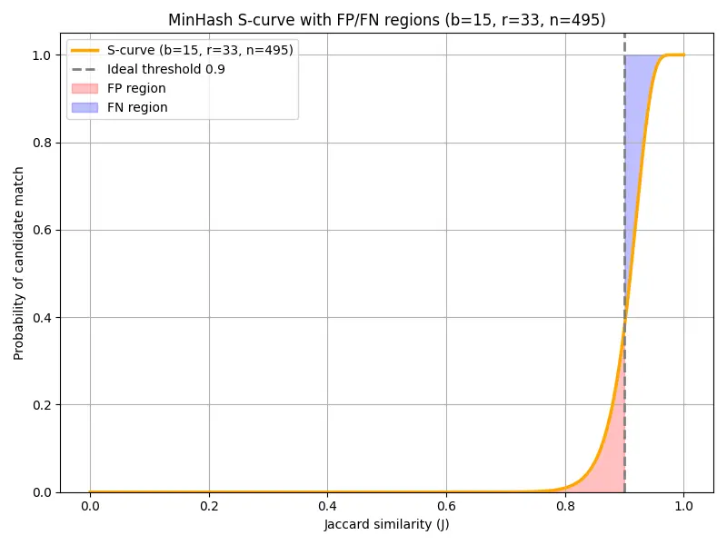
Breaking down the error regions of this graph:

False positives (red): Messages with less than 90% similarity but match in at least one band. For this configuration the cumulative error (fp_area) shows a total area of 0.0108.

• The secondary check on the full fingerprint to recalculate the full Jaccard index on matching fingerprints eliminates false positives, but at the cost of additional computation time.
• Since these are easy to correct, a small amount of false positives from the band check is tolerable but each increases total search latency.

False negatives (purple): Messages with greater than 90% similarity but do not match in any bands are misses for a similarity lookup. For this configuration, the cumulative error (fn_area) shows a total area of 0.0163.

• Unlike false positives, negatives are misses that can’t be corrected. This is the worst kind of failure mode for this approximation. When choosing between minimizing FPs or FNs, we should err on the side of minimizing FNs!
• If optimizing for just minimal FNs within our top 10 list, we could end up with a different ideal configuration, such as $b = 16, r = 30$.

Other regions (white): Messages are properly included or excluded from the 90% similarity search. In these regions, our banding technique is working perfectly to only find the right matches!

Implementing similarity lookup with a database

Finally, we have all the necessary pieces in place to build a solution that can efficiently find matching messages at scale, and can easily be scaled horizontally by subdividing the set of messages.

First, the message is preprocessed. Using tokenization, shingling, and namespaces, every message is converted into a set. Once this set is constructed, MinHash creates a fingerprint of fixed size $n$, which is then split into $b$ bands.

Once the fingerprint and bands are calculated, the message can be stored for efficient retrieval with a band → message mapping. This mapping fits neatly in an inverted index. A database like Postgres, could leverage GIN for an inverted index, making the schema simply:

CREATE TABLE message_similarity_lookup (
	id UUID PRIMARY KEY,
	bands       []BIGINT,
	fingerprint []INT
);

CREATE INDEX ON message_similarity_lookup USING GIN(bands);

Searching for similar messages is easy with the above schema. Once fingerprints are known for a message, we efficiently find all candidate messages with matching bands, then filter those results further by calculating the approximate Jaccard index on the complete fingerprint. The retrieval query for the above schema is:

-- Parameters:
-- $1 ([]INT): Input bands
-- $2 ([]INT): Input fingerprint
-- $3 ([]INT): Input Jaccard threshold

SELECT
	message_id
WHERE
	-- Indexed lookup on bands, matching the S-Curve for recall
	bands && $1
	
	AND
	 
	-- Calculate jaccard on the full fingerprint by counting matching pairs
	(
		SELECT COUNT(*)
    FROM generate_subscripts(fingerprint, 1) AS i
    WHERE fingerprint[i] = $2[i]
	) >= ($3 * array_length($2))

Finally, another table can track membership of messages in groups. This enables similarity search to perform live clustering of messages and makes it easy to join a group from a known message, or to find all messages in a group. Live clustering of messages and tracking the membership of messages and groups is the final piece that connects similarity search to message grouping at Sublime.

CREATE TABLE message_group_member (
	message_id UUID PRIMARY KEY
	group_id UUID
);

CREATE INDEX ON message_group_member(group_id);

Recap and wrap

To quickly recap, by initially representing messages as a collection of string fields, we learned why edit distance is hard to scale and how set similarity enables efficient comparisons. After deploying tokenization and shingling to define sets, we next used MinHash for consistent sampling to construct fixed-length fingerprints. Finally, we leveraged banding for fast similarity lookup at high scale.

This lookup approach turns the abstract math of Jaccard and MinHash into a tangible, practical tool for live clustering that meets tight latency requirements and enables grouping over millions of messages in milliseconds. And I said in the opening, message grouping then enables some very powerful features within Sublime.

If you enjoyed this post, send us your questions and comments over social (LinkedIn, X). And if this is the type of challenge you like tackling, get in touch with our Engineering team.